Lab 10: Dipole Moments and Electric Flux

We started the day talking about the path an electron will take if it undergoes between a positive plate and a negative plate. The result was a projectile motion trajectory. In addition, the acceleration is on the direction of the electric field.

We also looked into electric dipole in an electric field, which is defined as p = 2aq. In the dipole moment the vector is directed from the negative charge towards the positive charge. We also derived torque as the result from the cross product between the dipole moment and the electric field. Also, we found that the work is the negative dot product between the dipole moment and the electric field, so the electric potential energy should be just the dot product.

This picture describes the removal of makeup at the physics level.

We also worked in a Vpython program, which consisted on displaying the electric field due to two charges.

 Here is the code.

Here is the output of the electric field.

Then we started using the caltech electric field applet in order to have a visualization of the electric field due to various point charges.

One electron and it's electric field.

This picture shows the electric field of a positive charge with a negative charge.

Here professor Mason put a point charge for us to determine the direction it will take.

Professor Mason introduced to us an example of flux model. He explained with a square wire that if it is parallel to the wood surface then the flux will be max since it covers the maximum amount of electric field vectors; likewise, if the wire is perpendicular to the surface then the flux is zero.

This photo shows that the flux is maximized.

We determined the flux to be the dot product between the area and the electric field.

We did an example that consisted on finding the flux of a box when the electric field vectors are going to the positive x direction. 

Lab 9: Electrical Field

Today we started the day by talking about the similarities about gravitational force and electric force.

With these similarities we were able to determine the second law of electrical field. F = qE.

 We also talked about positive and negative charges, if the charge is positive then it acts on the direction of the electric field, meaning that the electric field moves away from the positive point charge. If the point charge is negative then the electric field moves in the direction of the charge.

 Here, we defined step by step, how will we represent an electric field of a single charged particle into VPython.

 This is the code we used to fix the arrows direction. Before all the arrows point to the positive x direction.

 This was our visual prediction of the sample code provided by Professor Mason.

Professor Mason introduced to us the Superposition Principle which says that the electric field is just the sum of all the electric fields. We did an example using this principle.

 Professor Mason added another point charge, and these are the calculations for that point charge.

 Then we worked in an exercise that consisted on dividing a uniformly charged rod into 10 pieces, and see what would the result be in each piece due to a point charge.

An example that consisted on deriving the electric field using changes in length.

We used excel to calculate the total electric field of all 10 pieces.

Computational Modeling: VPython

Our first assignment was to watch youtube video referring the use of the compiler VPython, and develop some basic designs.

This is the source code to display spheres and arrows.

 This is the output of the source code above.

 This was the second assignment that consisted of assigning attributes to each variable so that we could therefore improve the style of coding and perform more operations

 This is the output of the source code above, connecting each ball by using the relative position vector.

 This is the result of moving one sphere twice its y-distance. The result of that caused the arrows to change, from big to small.

 By using the command, print(variable.attribute), we can see that it prints our desired variable's coordinates into the shell windows.

Lab 8: Electric Charge and Force

We started the day with a ballon experiment. Rubbing the ballon with hair will make the ballon to stay on the glass surface because when the ballon is rubbed it becomes a charged object, and when it stays on the surface of the glass, we know that both the balloon and the glass have opposite charges that attract each other.

 Here is our prediction of both cases. However, we could not see the second case to work effectively due to the climate. The second case consisted on rubbing the balloon with silk, it supposes to also stay on the glass surface.

 We conducted an experiment about interactions between scotch tape strips. First with two strips pasted on the table, we were to supposed to peel them off and cause and interaction with each other and see what the final result will be.

This video shows that both scotch strips repel each other, the reason is because both have the same charges when pulled off the table.

This is an example of just 1 scotch strip pasted on the table making interaction with a new scotch strip, and as we can see both attract each other due to the difference in charges.

 Then we placed two strips of tape on the table sticky side down and labelled them as B, also we placed another two strips on top of them.

 The results were that, T and T repelled each other, B and B repelled each other also, but T and B attracted each other.

 We worked on this problem example after watching a video of two magnetic balls. When a magnetic ball gets closer to the hanging ball, it moves apart. So we find the angle as a function of the length of the rope and the distance is moved, which is θ = arcsin(X2/L). Then we found the force acting on the ball. F = mg(tanθ). Then we substituted θ in order to get  F = mg(tan(arcsin(X2/L)), which will be needed for the next experiment.

 We started working on the Coulomb electric force law video. This is our data and graph after doing what was asked in the lab manual. We fit our curve with an inverse function of degree two.

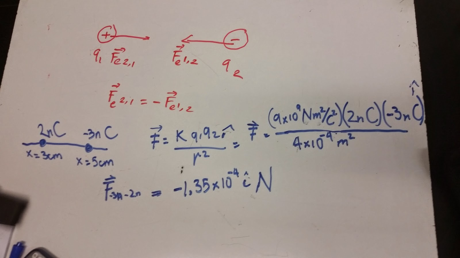
 We work on an example using Coulomb's Law.

 We decomposed the force into x and y components.

We conducted an experiment using the Van De Graff generator. When is turned on, the paper streamers start to float on the air because they have the same charge. Here we put a pie pan on top of it, when we turned the machine on, it flew away.

In this video we can see that if you put your hand on the Van De Graff generator, you will get electric charges. Also, when the hand was taken away, the paper strips started to float.

We put a Franklin motor on it.

 The charges generated by the device are spread out until it reaches the top of the Franklin motor, causing it to rotate. The strips don't float anymore because all the charges go to the motor.

Finally, we used Coulomb's law and the Universal Gravitation law in order to find the ratio of forces between them. Our result was 4.182x10^42.

Conclusion

Here are the answers to the conclusion section.

Lab 7: Entropy, Stirling Engine, Coefficient of Performance, and Bubbles

We started the day talking about the main difference between auto cycle and diesel cycle. Diesel cycle can keep on compressing until the gas ignites, allowing a constant pressure process. Also, it is more simpler and has more effectiveness compared to auto cycle since you can get more work per cycle. Diesel engines try to inject fuel at the very last second in order to achieve instantaneous ignition.

We learnt a new term, entropy, which is the amount of heat energy absorbed over the thermal energy. Also the second and third law of thermodynamics was introduced to us, which define that entropy can be created but not spontaneously destroyed, and it is the entropy (not energy) of a system that goes to zero as the absolute temperature goes to zero, respectively.

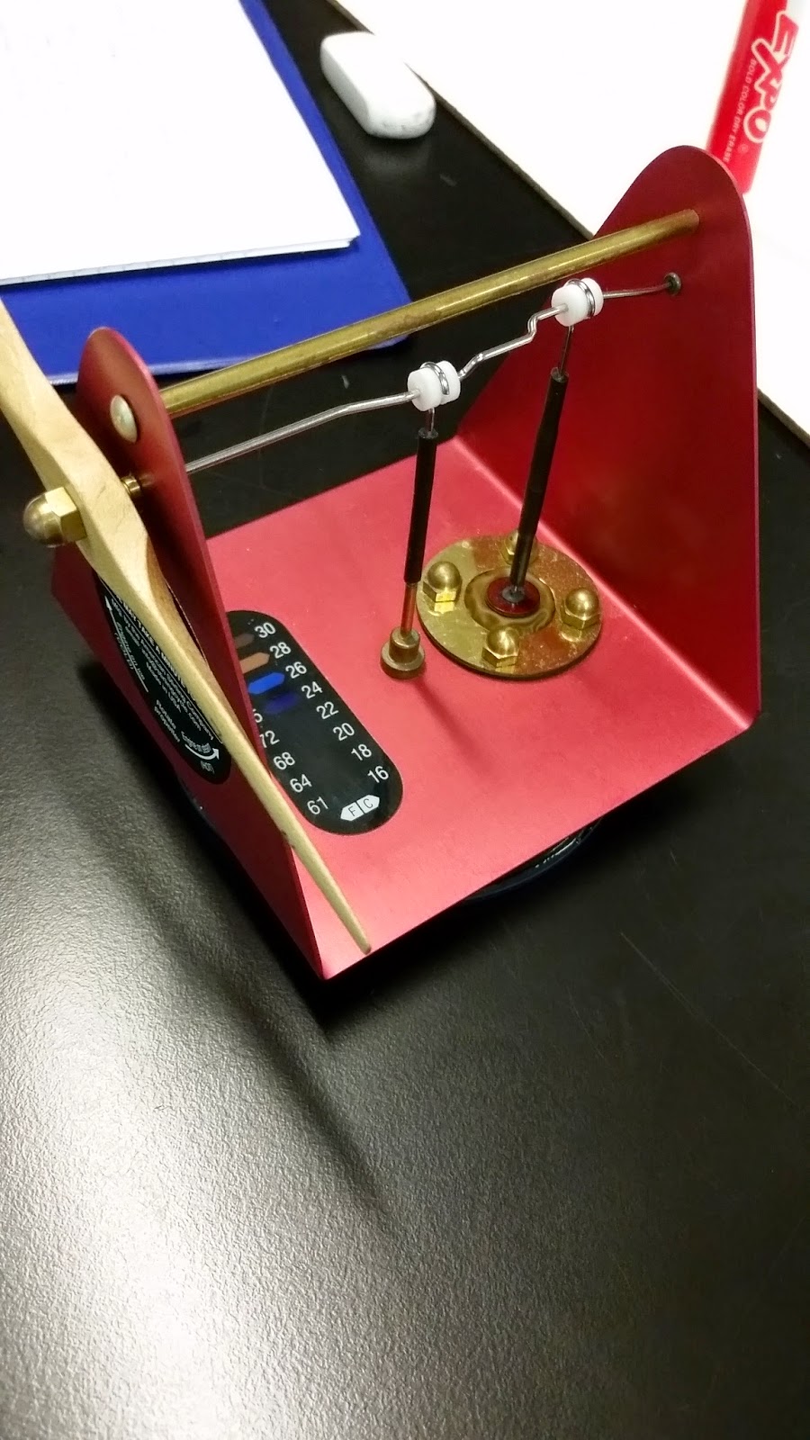
We also worked on a stirling engine cycle, which is another real gas cycle. It is used to run very slow. Fast cycles are adiabacs, and slow cycles are isotherms, which are used to generate electricity. First we conduct a experiment in which the hot reservoir was located at the bottom of the apparatus while the cold reservoir was on the top side of the apparatus.

Here is a video that shows how the stirling engine works, when the bottom is hot and the top is cold. The revolutions per second increases as the temperature difference increases. In this case the fan rotates counterclockwise.

Then professor Mason, reverse the temperatures, by using ice to cold the bottom side, and add hot water to the top side of the apparatus. Causing the fan to rotate clockwise.

Here is a video of reversing the temperatures. We can see, when professor Mason tries to make the fan spin counterclockwise, the fan just goes clockwise.
Stirling engines generates double the electricity compared to solar panels.

Here we calculated the efficiency of the stirling engine cycle.

Professor Mason introduced the idea of coefficient of performance, which is the ratio of the heat removed over the work. Also the maximum coefficient of performance is give by the ratio of the temperature of the object over the difference in temperature of the outside and the object. In this example we used the maximum COP to find the heat of the refrigerator.

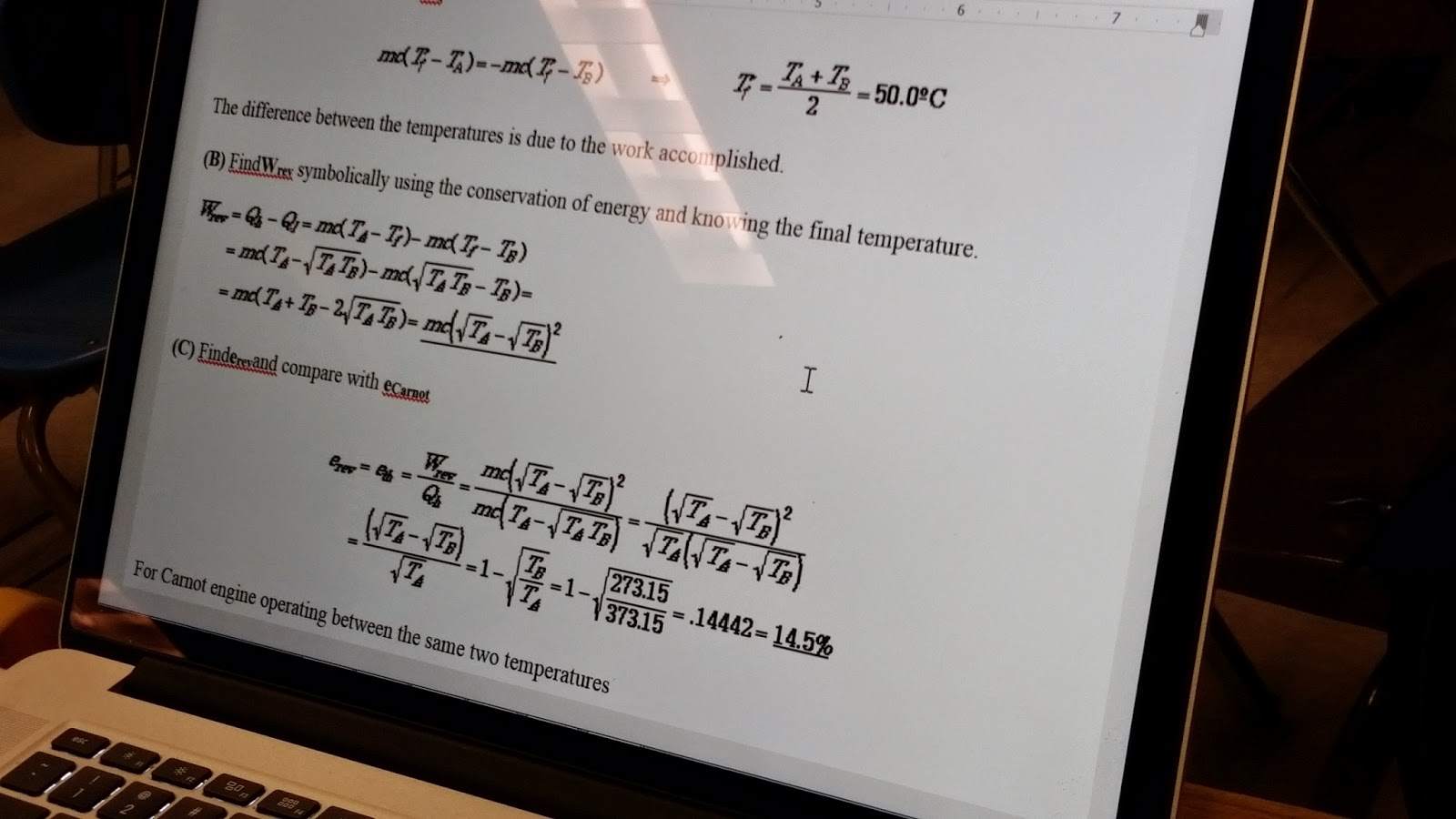
Here is an example of the effectiveness of a heat engine, which is the ratio between the actual output over the maximum output of energy by reversible process.

This was another working example of effectiveness.

This was a refrigerator freezing ice problem that consisted on finding the maximum COP and the time to freeze 4.2kg of water at 18 degree Celsius.

Then we conducted an experiment about bubbles. First when professor Mason blowed through the apparatus the bubbles fell down.

In this video we can see that when the bubbles are blown by natural gas, then they tend to go up.

This video shows that if you burn the bubbles made of natural gas, they will burn.

Here is professor Mason playing with fire.